SALDA for timelapse microscopy
This project is maintained by amsikking from Calico Automation, and was funded by Calico Life Sciences LLC
Appendix
Note that this is a limited PDF or print version; animated and interactive figures are disabled. For the full version of this article, please visit one of the following links: https://amsikking.github.io/SALDA_for_timelapse_microscopy
A simple automatic liquid dispense arrangement (SALDA) for timelapse microscopy
Multiwell samples
Multiwell samples are somewhat varied in size and specification so it can be challenging to foresee and accommodate all options. However, we found that most of our users were using either chambered coverslips or multiwell plates in the following formats:
| Format | Well size (mm) | Well spacing (mm) | Vol. (μl) | Coverslip (μm) |
|---|---|---|---|---|
| Cellvis 8 well chambered | 9.3 x 8.9 x 10.8 | 11.52 x 11.04 | 889 | 170 ± 5 glass |
| Cellvis 8 well chambered (short) | 9.3 x 8.7 x 10.8 | 11.57 x 11.20 | 874 | 170 ± 5 glass |
| Cellvis 18 well chambered | 6.1 x 5.7 x 10.8 | 7.56 x 7.14 | 369 | 170 ± 5 glass |
| Cellvis 18 well chambered (short) | 6.1 x 5.7 x 10.8 | 7.56 x 7.14 | 370 | 170 ± 5 glass |
| Cellvis 96 well plate | 6.2 x dia x 11.9 | 9.00 x 9.00 | 361 | 170 ± 5 glass |
| Cellvis 384 well plate | 3.3 x 3.3 x 11.4 | 4.50 x 4.50 | 124 | 170 ± 5 glass |
| Ibidi 8 well chambered | 10.7 x 9.4 x 6.8 | ? x ? | 684 | #1.5 polymer |
| Ibidi 8 well chambered (high) | 10.7 x 9.4 x 9.3 | 12.20 x 10.90 | 935 | 170 ± 5 glass |
| Ibidi 18 well chambered | 6.1 x 5.7 x 6.8 | 8.10 x 7.45 | 236 | 180 polymer |
| Revvity 96 well plate | 6.4 x dia x 12.7 | 9.00 x 9.00 | 408 | 200 ± 10 polymer |
| Revvity 384 well plate | 3.3 x 3.3 x 12.9 | 4.50 x 4.50 | 137 | 200 ± 10 polymer |
So in practice the usable volumes range from ~100 μl to ~900 μl and the well heights from 6.8 mm to 12.9 mm (the max overall height goes up to 14.35 mm for Revvity well plates).
Fluidic connectors
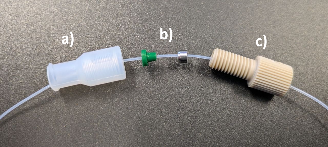
We use a Luer adaptor (IDEX P-648), ferrule (IDEX P-248X) and nut (IDEX P-255) to make a reliable connection between the delivery tube and the syringe. Simply slide the parts onto the delivery tube and firmly tighten the nut onto the Luer adaptor with fingers (Figure A1).
Note: the ferrule permanently binds to the tube and cannot be easily moved or removed. So it's important to place the ferrule in the correct location before final tightening (i.e. at the end of the tube, either flush or with a small amount protruding).
Delivery tubes
We tested delivery tubes with different dimensions, materials and terminations, with both water and media to reach a preferred configuration.
Preferred delivery tubes
| ID | Type (part) | OD (in) | ID (in) | OD (mm) | ID (mm) | Termination |
|---|---|---|---|---|---|---|
| 1 | PTFE AWG 30 (Zues SWTT-30-C) | 0.030 | 0.012 | 0.762 | 0.305 | clean 90° cut |
| 2 | PEEK natural (IDEX 1568XL) | 1/32 | 0.015 | 0.794 | 0.381 | clean 90° cut |
In general the PTFE tubing (1) is preferable for many applications due to it's lower cost, excellent chemical resistance and higher water contact angle which results in more accurate dispenses (especially for 'sticky' liquids). However, the PEEK tubing (2) is a solid backup with greater stiffness, strength and wear resistance, and is typically made to tight tolerance. Both materials can operate at high temperatures (~260°C).
Tested delivery tubes
| ID | Type (part) | OD (in) | ID (in) | OD (mm) | ID (mm) | Termination |
|---|---|---|---|---|---|---|
| 3 | PTFE AWG 32 (Zues SWTT-32-C) | 0.020 | 0.010 | 0.508 | 0.254 | clean 90° cut |
| 4 | PEEK natural (IDEX 1568XL) | 1/32 | 0.015 | 0.794 | 0.381 | clean 45° cut |
| 5 | PEEK natural (IDEX 1568XL) | 1/32 | 0.015 | 0.794 | 0.381 | squashed 90° cut |
| 6 | PEEK blue (IDEX 1581L) | 1/32 | 0.010 | 0.794 | 0.254 | clean 90° cut |
| 7 | PEEK red (IDEX 1576L) | 1/32 | 0.005 | 0.794 | 0.127 | clean 90° cut |
From the results of the preferred PTFE tubing (1) it seemed like PTFE tubing with an even smaller outer diameter (OD) and slightly smaller inner diameter (ID) could be even better (3). However we found that 3 was overly flexible and couldn't adequately carry the high syringe pump pressure from the small ID, giving a slower and less accurate response than 1. Configuration 4 is the same as configuration 2 but with a 45° cut and was worse (likely due to the increased surface area).
We tried 'squashing' the natural PEEK tubing at the end with flat pliers (5) to make a less favourable geometry for the retained droplet (i.e. strongly elliptical instead of circular). This actually worked quite well since the PEEK material was able to retained to squashed shape and the smallest accurate dispense volume was reduced from 10 μl to 4 μl with water. However we found that the squashed termination caused significant 'foaming' with media and was therefore not attractive for imaging.
We tried small ID PEEK tubing in blue (6) and red (7) guage but the greatly increased pressure resulted in slower dispense speeds and lower accuracy, especially for the red tubing. We also tried natural peek tubing (2) with a short termination in either blue (6) or red (7) tubing but this inceased complexity for no obvious gain.
Fluidic resistance
A useful concept when designing fluidic systems is the idea of the 'fluidic resistance' of the system \( R_H \). In general, for a given a flow rate \( Q \) the pressure drop across the system \( \Delta P \) is directly proportional to the fluidic resistance [Tipler 2003]:
\[ \Delta P = Q R_H \tag{a1} \]So for a given flow rate a higher fluidic resistance will give a higher drop in pressure, and a lower fluidic resistance a lower drop in pressure. Usually a system can only deliver (or tolerate) some maximum amount of pressure, and there is often a minimum flow rate that is required, so this puts bounds on how much fluidic resistance is acceptable for a particular application. In the special case of a cylindrical tube under laminar flow we can calculate the fluidic resistance directly with the Hagen-Poiseuille equation [Tipler 2003]: \[ R_H = \frac{8 \mu L}{\pi r^4} \tag{a2} \] Where \( \mu \) is the dynamic viscosity of the fluid (~ 0.001 Pas for water at room temp.), \( L \) is the length of the tube and \( r \) is the inner radius of the tube. So the fluidic resistance of a tube is directly proportional to the length of the tube and inversely proportional to the fourth power of the inner radius (i.e. twice the length is twice the resistance and half the radius is 16 times the resistance!).
Mechanical design
Here we present the full mechanical design for this implementation of a SALDA, with examples of how to bend stainless steel tubes to hold the delivery tube, an XYZ kinematic arm for positioning the delivery tube, an Okolab stage top incubator and custom riser to accommodate the delivery tube, and a syringe pump mount to reduce the length of the delivery tube. Although the CAD presented here is specific to an Okolab stage top incubator and a Leica DMi8 microscope, we expect the design and associated methods are readily modified and adapted to any microscope platform that can accommodate a small diameter tube (~2 mm).
Bending stainless steel tubes
To keep the mechanical design simple, low cost and adaptable we figured out how to bend small diameter stainless steel tubes to hold the otherwise flexible delivery tubes in place. We found that two small radius 90° bends were useful for our immediate implementation. One 90° bend above the sample to direct the delivery tube into the sample well and a second 90° bend on the clamped end to stop unwanted rotation of the stainless steel tube (shown in Figure 5 of the main text).
When attempting a small radius bend in tubing the 'bend factor' \( f \) is a helpful concept, defined as the ratio of the center line radius \( CLR \) to the outer diameter of the tube \( D_{OD} \):
\[ f = \frac{CLR}{D_{OD}} \tag{a3} \]A minimum bend factor of 2 is recommended for many materials, with 3 or more being safer to avoid distorting the tube while bending.
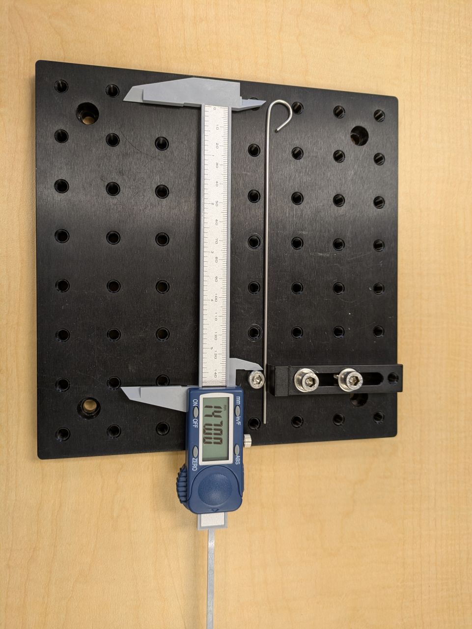
We tried bending 8" long stainless steel tubes with outer diameters of ~1.7 mm, ~1.8 mm, ~2.1 mm and ~2.4 mm mm around an M6 socket head bolt (~5 mm radius), which gave bend factors in the range of ~2.6 to ~3.5. To do this we used finger strength to bend the tubes on a simple jig made from an aluminium breadboard (Thorlabs MB2020/M) with a table clamp (Thorlabs CL2M) and 3 M6 socket head bolts (Figure A2). In practice we found that the 1.8 mm tubing with a bend factor of ~3.3 was well behaved and that bend factors much lower than this could collapse the tube. The inner diameter (~1.4 mm) of the 1.8 mm tube is also large enough to readily thread in the delivery tubes, and stiff enough to achieve repeatable XYZ positioning without being overly large. Larger tubes are easier to thread and stiffer but are harder to accommodate in the otherwise tight opto-mechanical design.
| Step: |
XYZ kinematic arm
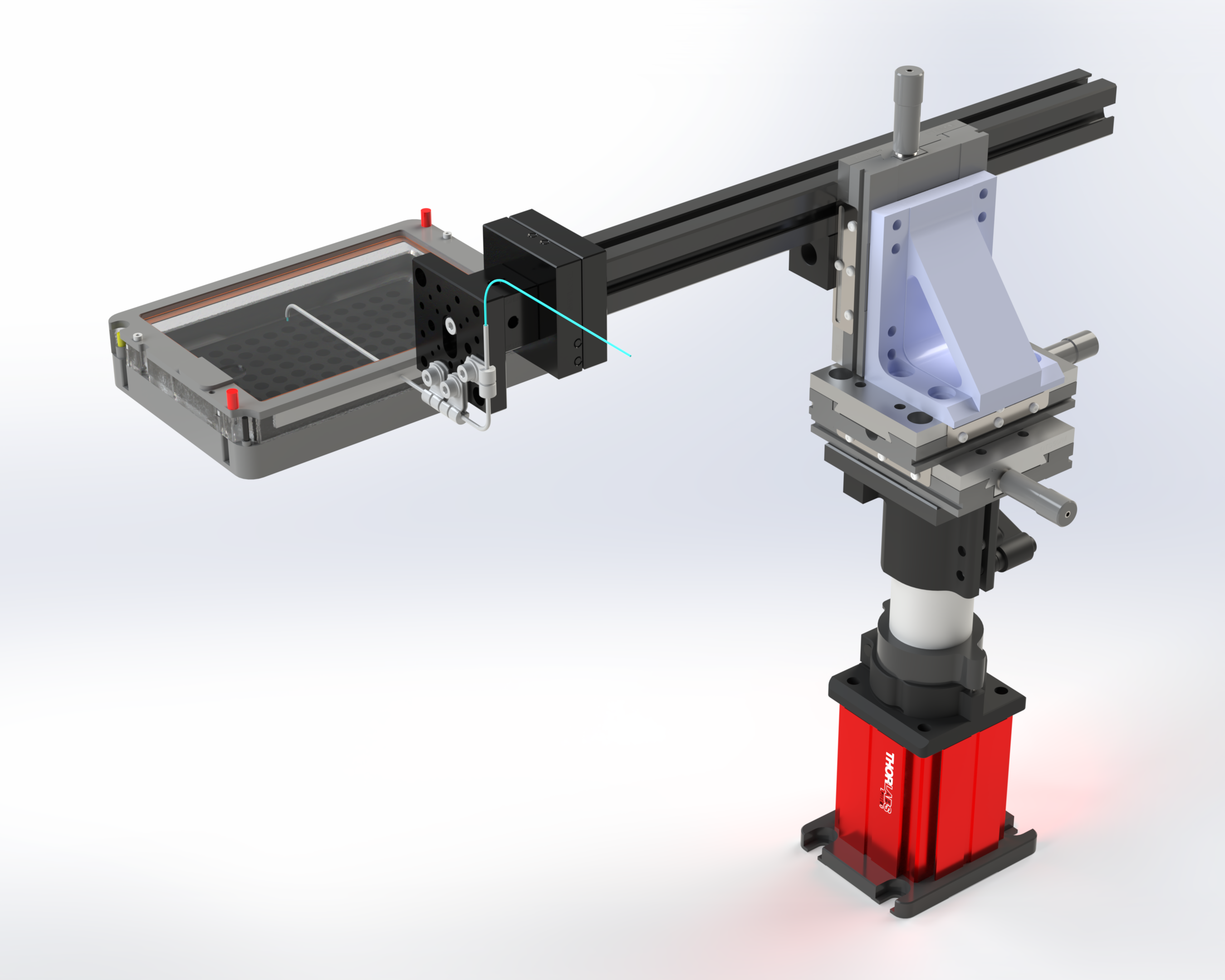
Here's an example of a SALDA with an XYZ kinematic arm for positioning the delivery tube above the objective (Figure A3). This particular arrangement works well with a Leica DMi8 inverted microscope but we expect the same or similar versions to work well with other microscope platforms (CAD here).
Okolab stage top incubator
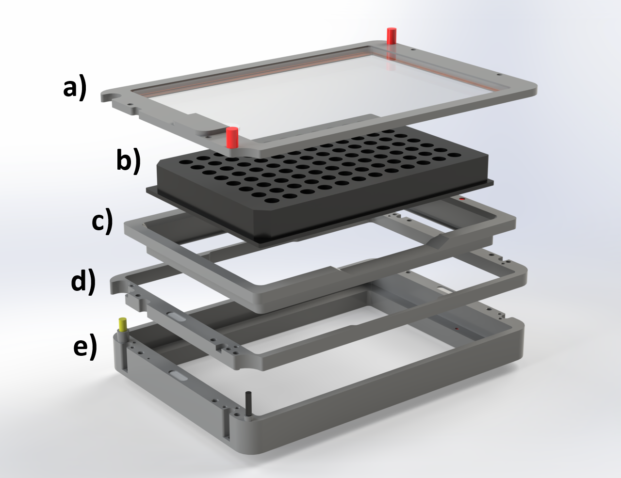
Here we chose to integrate a SALDA with an Okolab H301-K-FRAME stage top incubator that has built in temperature, CO2 and humidity control to provide a stable environment for long time lapse microscopy of living cells and organisms. To allow the SALDA delivery tube to enter the incubator we needed to modify the H301-K-FRAME assembly. Fortunately, the H301-K-FRAME has an intermediate 'riser' part that can easily be removed (Figure A4, d)) and replaced with a custom riser.
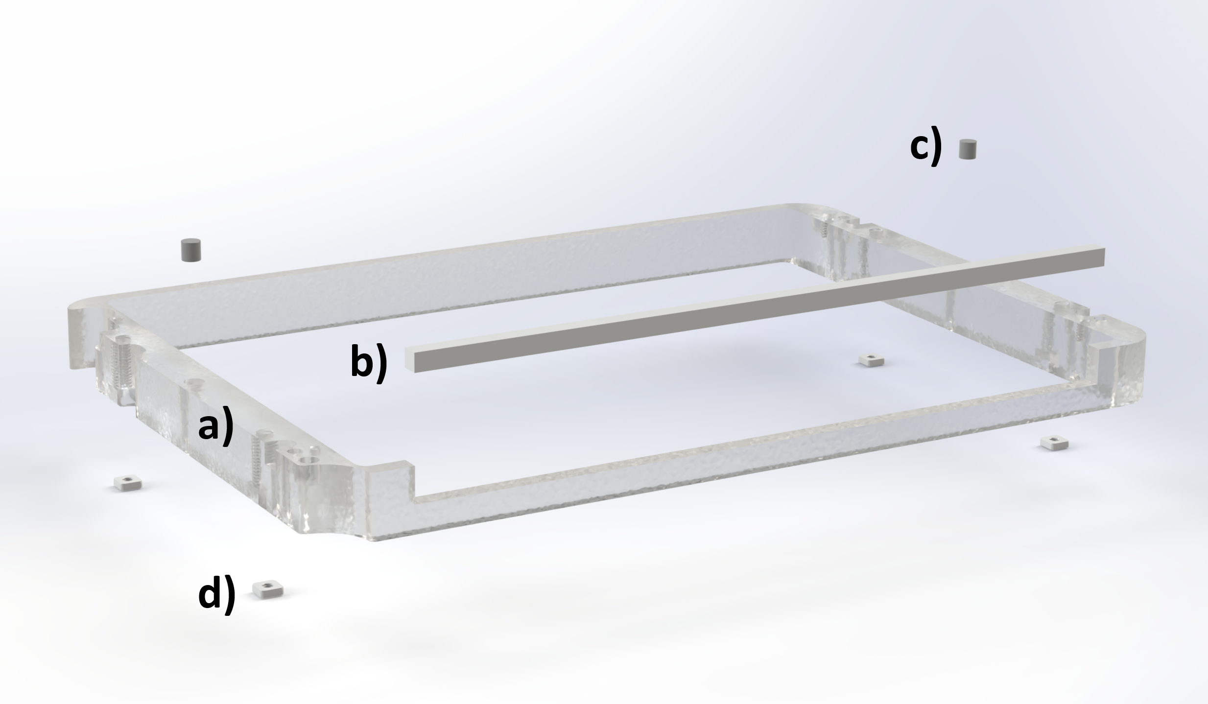
Okolab stage top incubator custom riser
We designed a custom riser for the Okolab H301-K-FRAME stage top incubator (CAD here). This new part adds height to the lid and has a cutout to add some flexible seals to allow the SALDA delivery tube to enter the incubator (Figure A5). The cutout extends to the length of a standard multiwell plate to allow the delivery tube access to all the wells as the microscope XY stage moves around. We opted to 3D print the riser with a Formlabs Form 4 MSLA printer, using their 'Clear V5' photopolymer resin (takes about 2h). However, this part could also be machined out of aluminium or other plastics. We glued the magnets and square nuts in place using Gorilla clear 5min two part epoxy.
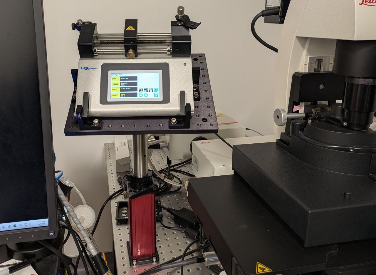
Syringe pump mount
We designed and built a basic syringe pump mount for the KDS Legato 110 syringe pump (CAD here). This mount is optional but holds the syringe pump securely in a convenient location near the sample which reduces the length of the delivery tube and therefore the liquid pressure in the system (Figure A6). We expect the same or similar designs to be helpful with other syringe pump models and microscope platforms.
Trueness and precision
To benchmark a SALDA we adopted definitions for 'accuracy', 'trueness' and 'precision'. High trueness is when the average measured value is close to the target value (i.e. a low systematic error). High precision is when the measured values are close to each other (i.e. a low random error). High accuracy is when both the trueness and precision are high.
Trueness
We equate high trueness to a low systematic error, which we can express mathematically as a low percentage error or low relative bias \( RB \):
\[ RB{(\%)} = 100 \left( \frac{\bar{x} - x_T}{x_T} \right) \tag{a4} \]where \( x_T \) is the target value and \( \bar{x} \) is the mean of \( N \) individual measurements \( x_i \):
\[ \bar{x} = \frac{1}{N} \sum_{i=0}^N x_i \tag{a5} \]Precision
We equate high precision to a low random error, which we can express mathematically as a low coefficient of variation \( CV \):
\[ CV{(\%)} = 100 \ \frac{\sigma}{\bar{x}} \tag{a6} \]where \( \sigma \) is the standard deviation of the measurements:
\[ \sigma = \sqrt{\frac{\sum_{i=0}^N |x_i - \bar{x}|^2}{N}} \tag{a7} \]Retained Droplet
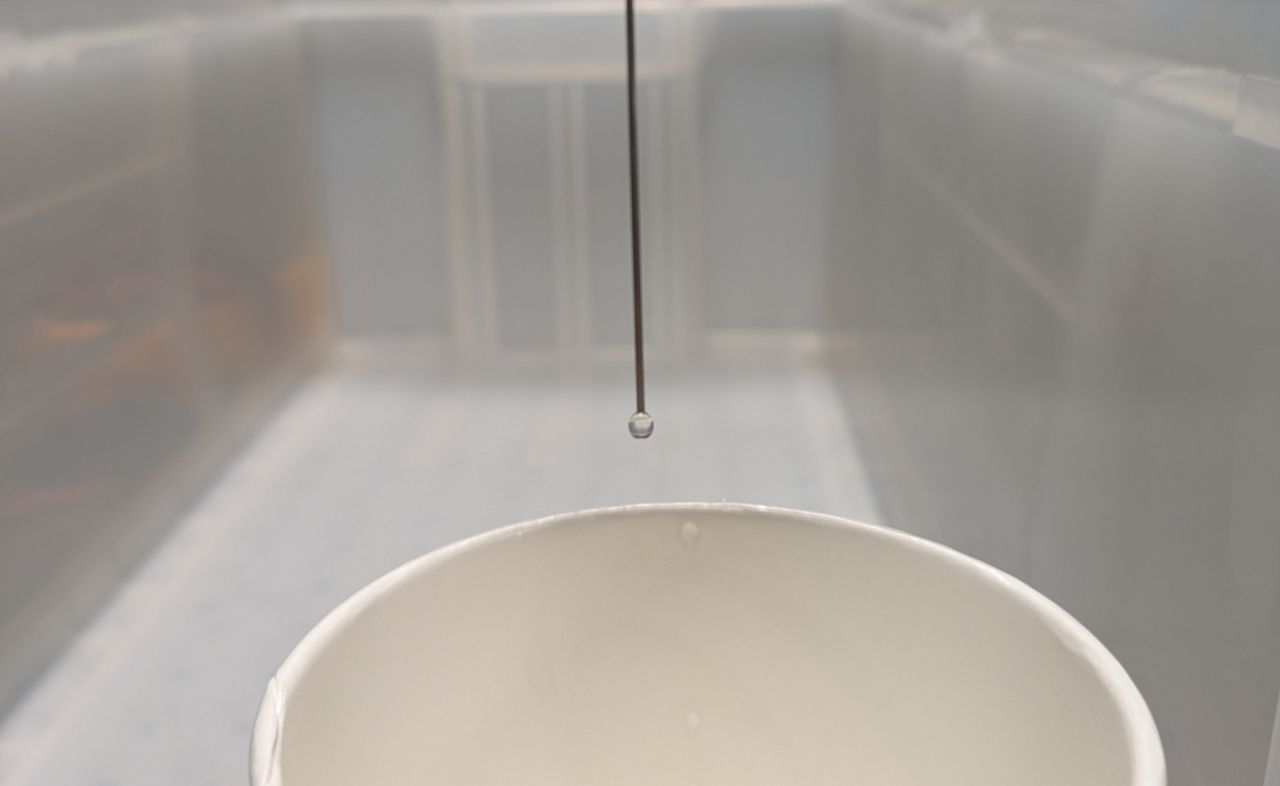
We found an unwanted 'retained droplet' (RD) would form on the end of the liquid delivery tube through surface tension counteracting the force of gravity pulling the liquid downwards. The size of the RD would determine the smallest liquid dispense volume we could attempt, so a smaller RD would enable smaller dispense volumes and a larger RD would limit a SALDA to larger dispense volumes (Figure A7).
Gravimetric test rig
To evaluate the accuracy of a SALDA we needed a way to measure the dispensed volumes and compare them against the requested or target dispense. To do this we adopted a simple 'gravimetric' approach where we used an analytical balance (Ohaus EX225DAD) to measure the mass of a cup before and after a dispense operation and used the change in mass to estimate the dispensed volume (Figure A8).
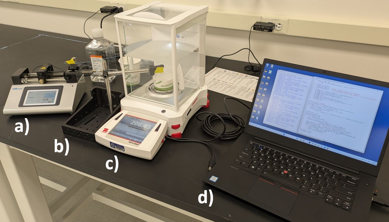
We wrote a flexible test program to configure the syringe pump (flow rate, direction and target volume) and measure the net weight of the dispense from the analytical balance. In practice we ran either fixed volumes (e.g. 10 μl) or random volumes in a given interval (e.g. 10 μl to 100 μl) for up to 100 iterations. A 5 second delay was included between the dispense and mass measurement to allow the fluidics and analytical balance time to stabilize. The idea of multiple 'shots on target' was explored at one point but ultimately not needed and so all the data presented here is single shot. Here's an extract of the test program showing the configuration and main loop:
# Configure syringe:
syringe_volume_ul = 2500
dispensed_volume_ul = 0

# Configure syringe pump:
flow_rate_ulps = 110 # max ~110 ul/sec for 2.5ml glass syringe (6.62764 ml/min)
sy_pump.set_flow_rate('withdraw', 'max', None)
sy_pump.set_flow_rate('infuse', flow_rate_ulps, 'ul/sec')
sy_pump.set_run_direction('infuse')

# Configure:
target_volume_ul = 10   # 10-100 typical
random_volumes = False
random_volume_range = (10, 100)
iterations = 100 # how many iterations?
shots_on_target = 1 # how many shots are needed for high trueness? prefer 1

# Get unique filename and start weight:
dt = datetime.strftime(datetime.now(),'%Y-%m-%d_%H-%M-%S')
filename = dt + '_volume_vs_weight.csv'
previous_weight_mg = float(balance.get_immediate_weight()[0])
for i in range(iterations):
    print('\niteration = %i (dispensed_volume_ul=%s)'%(i, dispensed_volume_ul))
    if random_volumes: # change target volume if random:
        target_volume_ul = np.random.randint(low=random_volume_range[0],
                                             high=random_volume_range[1])
    # update total dispsensed volume and exit if syringe is empty:
    dispensed_volume_ul += target_volume_ul * shots_on_target
    if dispensed_volume_ul >= syringe_volume_ul:
        break
    sy_pump.set_target_volume(target_volume_ul, 'ul')
    # get data:
    for shot in range(shots_on_target):
        print('\nshot = %i'%shot)
        sy_pump.set_run_direction('infuse')# forces volume update? device error?
        sy_pump.run()
        time.sleep(5) # wait for fluidics and balance to stablize
        immediate_weight_mg = float(balance.get_immediate_weight()[0])
        net_weight_mg = round(immediate_weight_mg - previous_weight_mg, 2)
        previous_weight_mg = immediate_weight_mg
        with open(filename, 'a', newline='') as file:
            writer = csv.writer(file)
            if i == 0 and shot == 0:
                writer.writerow([ # write headers
                    'shot','flow_rate_ulps','target_volume_ul','net_weight_mg'])
            writer.writerow([ # write data:
                shot, flow_rate_ulps, target_volume_ul, net_weight_mg])
Adherent cells
U2-OS cells were maintained in DMEM (Thermo Fisher #31053028) containing 10% FBS (Gibco #26140-079), 1 mM sodium pyruvate, and 2 mM GlutaMAX in a 37°C incubator with 5% CO2. Cells were passaged every 2-3 days by trypsinization with TrypLE express dissociation reagent. Cells were routinely tested for mycoplasma contamination and were discarded after 20 passages.
For imaging experiments, 8 well chambered coverglass (CellVis) were coated with bovine fibronectin (Sigma) diluted 1:100 in PBS for 1-5 hours at 37°C. Dishes were washed three times in PBS immediately before cell addition. U2-OS cells were seeded into chambered coverglass at 25,000 cells per well and allowed to adhere at room temperature for 30 minutes before transferring to the incubator. Cells were plated approximately 24 hours before imaging.
One to two hours prior to imaging, cells were media changed in complete culture media supplemented with 25 mM HEPES to reduce pH drift, along with 4 μM CalBryte 520 AM (AAT Bioquest) and 0.04% Pluronic® F-127. To remove excess dye immediately prior to imaging, media was exchanged to complete DMEM with 25 mM HEPES. Thapsigargin (Sigma ready made) was made up as a 1000x-10000x DMSO stock and diluted to a 3x working solution in complete media before loading into the glass syringe for addition.
Setup
In practice we found a SALDA straightforward to set up for an imaging experiment and well behaved. However there are some practical details that are worth considering:
- To load the syringe we found it most convenient to remove it from the syringe pump, disconnect the delivery tube with the Luer lock and manually load the syringe directly from the source (e.g. a conical tube). We would then reconnect the Luer lock, re-attach the syringe to the syringe pump and manually drive the syringe pump screw (using the arrow keys on the touch screen) to eject liquid into a waste container (i.e. to remove air and have it ready for a dispense).
- During the setup we think it's best to place the SALDA holding tube onto the magnetic mount with a dry end (i.e. no retained droplet) to avoid the risk of accidentally dropping liquid into the sample (i.e. by shaking loose droplets from the end of the delivery tube).
- Due to 2. it's helpful to have a spare (i.e. trash) well in the sample or an additional dish to the side that can be used to dispense a few times with the SALDA and get it 'primed' for the experiment.
- The XYZ kinematic arm is used to position the SALDA holding tube over the objective (XY) and at the right height (Z) so that the holding tube sits comfortably between the flexible seals on the incubation chamber (or otherwise in a good location for other setups). Final Z adjustments can be made by sliding the delivery tube towards or away from the sample before securing it with tape (e.g. Figure A2, 11)).
- To minimize artefacts from using a SALDA it's best to adjust the XY position of the holding tube away from the immediate field of view of the microscope, but not so far as to risk dispensing out of the well or into a neighbouring well. So extra care is needed when imaging close to the edge of a well or if running a tiling routine etc.
- Compared to manual pipetting, switching dispense liquids is slower and requires partial disassembly of the setup and flushing and cleaning the fluidics. This should be taken into account when planning experiments.