Any immersion remote refocus (AIRR) microscopy
This project is maintained by amsikking in the York lab, and was funded by Calico Life Sciences LLC
Appendix
Note that this is a limited PDF or print version; animated and interactive figures are disabled. For the full version of this article, please visit one of the following links: https://amsikking.github.io/any_immersion_remote_refocus_microscopy
Any immersion remote refocus (AIRR) microscopy
Theory
Here we present the equations used in the main article.
Numerical aperture and resolution
The numerical aperture (NA) is defined as: \[ NA = n_i\sin\theta_i \tag{a1} \] where \( n_i \) is the refractive index (RI) of the immersion medium and \( \theta_i \) is the collection half-angle of the objective. In the case of a planar RI boundary like a coverslip the NA is conserved via Snell's law: \[ n_s\sin\theta_s = n_i\sin\theta_i \tag{a2} \] where \( n_s \) is the RI of the sample and \( \theta_s \) is the collection half-angle in sample space. According to the Rayleigh criteria the smallest resolvable feature size \( r_{min} \) is then: \[ r_{min} = 0.61 \frac{\lambda}{NA} \tag{a3}\] where \( \lambda \) is the wavelength of the collected light [Pawley 2006].
Focal length, field of view and pixels
The objective lens focal length \( f \) is found with: \[ f = \frac{f_{TL}}{M} \tag{a4}\] where \( f_{TL} \) is the tube lens focal length (200mm for Nikon) and \( M \) is the magnification of the objective. The sample space field of view (FOV) is then assumed to be: \[ FOV = \frac{FN}{M} \tag{a5}\] where FN is the field number according to the manufacturer (20mm assumed for Nikon). When choosing an objective it can be useful to estimate the number of Nyquist pixels \( N_{px} \) the lens can deliver across the FOV using: \[ N_{px} = 2 \frac{FOV}{r_{min}} \tag{a6}\] Note: this can be useful for choosing a camera and also serves as a measure of the quality of the objective, where more pixels usually indicates a more sophisticated lens design (similar in concept to etendue).
Standard focus depth
From Sheppard 1991, equation 18 proposes that in a medium of refractive index \( n_1 \), the maximum acceptable wavefront aberration (Rayleigh criterion) will not be exceeded if the thickness of a slab of dielectric \( t \) and refractive index \( n_2 \) meets the following condition: \[ t \leq \frac{\lambda n_2^3}{2n_1^2(n_2^2 - n_1^2)\sin^4(\alpha/2)} \tag{a7} \] where \( \alpha \) is the collection half-angle in the \( n_1 \) space (i.e. the immersion). Originally evaluated for a phase error of \( \pi/2 \), equation \( (a7) \) gives negative values for \( n_1 \gt n_2 \). If we allow \( n_1 \gt n_2 \) and a phase error of \( \pm \pi/2 \) then we can rewrite \( (a7) \) in a slightly more convenient format to give the maximum depth of standard focus \( z_{sf\_max} \): \[ z_{sf\_max} = \frac{\lambda}{2\sin^4(\theta_i/2)} \left\lvert \frac{n_s^3}{n_i^2(n_s^2 - n_i^2)} \right\lvert \tag{a8} \]
Remote refocus depth
From Botcherby 2007, equation 23 proposes that the Strehl ratio \( S \) of a remote refocus can be modeled by: \[ S = 1 - \frac{4n^2k^2z^4(3 + 16\cos\alpha + \cos2\alpha)\sin^8(\alpha/2)} {75f^2(3+8\cos\alpha + \cos2\alpha)} \tag{a9} \] where \( n \) is the refractive index of the sample, \( k = 2\pi / \lambda \) is the wavenumber, \( z \) is the axial distance from the traditional focal plane, \( f \) is the focal length and \( \alpha \) is the collection half-angle of the objective. If we set \( S = 0.8 \) (the traditional diffraction limit) and rearrange we can estimate the maximum remote refocus depth \( z_{rr\_max} \): \[ z_{rr\_max} = \pm \frac{1}{2\sin^2(\theta_s/2)} \sqrt[4]{\frac{15 \lambda^2 f^2 (3+8\cos\theta_s + \cos2\theta_s)} {\pi^2 n_s^2 (3 + 16\cos\theta_s + \cos2\theta_s)}} \tag{a10} \] Note: the substitution \( \alpha = \theta_s \) is subtle. In Botcherby 2007 at the critical substitution of equation 8 (\( \sin\theta = \rho \sin\alpha \)) the paper reads "In this expression \( \alpha \) is the semi-aperture acceptance angle of the lens" so one could assume \( \alpha = \theta_i \). However the substitution is in reference to coordinates in object space.
Combined depth
For a microscope with remote refocus optics (e.g. Figure 2) we can now estimate the maximum focus depth in the sample \( z_{max} \) as the sum of the standard and remote depths: \[ z_{max} \approx z_{sf\_max} + \left\lvert z_{rr\_max} \right\lvert \tag{a11} \] Note: the approximately equals sign. The standard focus and remote refocus depths use different definitions for the diffraction limit, and are approximate models that ignore higher order aberrations. There is also no consideration given to field effects, chromatic aberrations or design and manufacturing imperfections that can be expected in real objective lenses.
Objective selection
In a SOLS microscope [Millett-Sikking 2019], as the half angle in the sample \( \theta_s \) decreases, the tilt of the last microscope \( \theta_{tilt} \) increases according to: \[ \theta_{tilt} = 90 - \theta_s \quad (deg) \tag{a13} \] Currently the AMS-AGY v2.0 objective [Yang 2022] has the most extreme tilt range of any SOLS compatible objective, with maximum tilt of 55 degrees. So combining \( (a1) \), \( (a2) \) and \( (a13) \) the minimum acceptable sample space NA is: \[ NA \geq 1.33\sin(90 - 55)= 0.76 \tag{a14} \] After applying the lower bound on NA of 0.76, the 'best' objectives for the standard immersions were selected in the following 2 categories:
-
Nikon objectives, highest NA:
Part # M NA Imm. WD (μm) FOV (μm) rmin (μm) N_px MRD70470 40x 0.95 air 210 500 0.342 2927 MRY10060 60x 1.27 water 180 333 0.256 2608 MRD73950 100x 1.35 silicone 310 200 0.240 1663 MRD71970 100x 1.45 oil 130 200 0.224 1787 -
Nikon objectives, most pixels:
Part # M NA Imm. WD (μm) FOV (μm) rmin (μm) N_px MRD70270 20x 0.80 air 800 1000 0.406 4930 MRD77200 20x 0.95 water 990 1000 0.342 5854 MRD73250 25x 1.05 silicone 550 800 0.309 5176 MRH01401 40x 1.30 oil 240 500 0.250 4005
Note: Speciality objectives in the categories of TIRF and Multi-photon may not perform optimally for RR and were avoided.
Zoom lens
In our previous RR designs we used static lenses to adjust the magnification between the sample and the remote space according to equation 2 [Millett-Sikking 2018, Millett-Sikking 2019]. Specifically we chose to modify the second tube lens in the optical train, often referred to as 'tube lens 2' or TL2. The TL2 location is convenient, as it leaves the first objective and tube lens pair in their traditional (stock) configuration, and allows the addition of a unity magnification scanning system. Here we take the same approach, and optimize our zoom optics at the TL2 location, specifying some of the upstream and downstream optics in order to produce a concrete design.
Specifications
To produce a zoom lens with stock parts we narrow the optical requirement to a specific RR system. We assume a standard microscope at 40x magnification since this offers many attractive primary objective options (air, water, silicone and oil immersion at high NA from various manufacturers). We then assume a 5mm focal length air lens for the second RR objective (often referred to as 'objective 2' or O2). For example the Nikon 40x0.95 air lens (9.5mm back focal plane diameter) is a good high NA option, with a high enough collection cone (~72deg) and pixel count (~2927) for most RR designs. We target a RR magnification that covers the full biological RI range (1.33-1.51) by tuning the focal length of TL2 in the range 150-132.5mm (i.e. 30-26.5x for microscope 2). Finally we assume a standard sCMOS field of view (~13.5mm width) and add the additional constraints of needing a constant track length and telecentric image.
Design
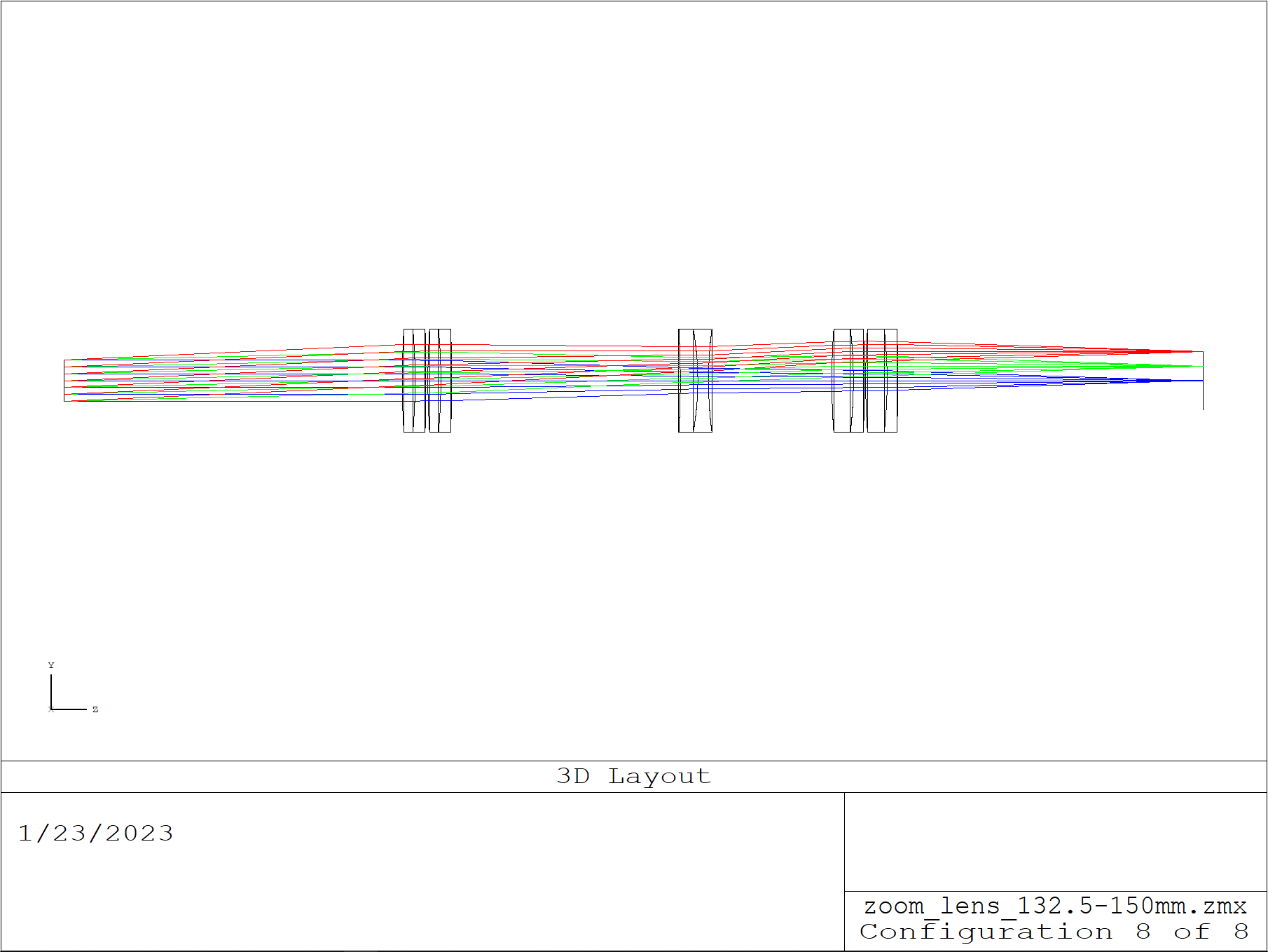
Using the above specifications, we adopt a simple 'positive-negative-positive' (PNP) zoom design and cycle through readily available stock parts. After some iteration we settle on a series of Edmund Optics achromats that satisfy our optical requirements, whilst also being mechanically compatible and inexpensive (see the mechanics section for parts). Our constraint of only using stock lenses forces a 5 achromat solution (Figure A2), where a 3 achromat custom design would suffice. We note that a 'standard' tube lens typically has 2 achromats, so a 3 lens solution would only add 1 achromat to the optical train (a minimal drawback for the system). However, we consider the small penalty on transmission efficiency (~1.5%) from the 2 additional achromats in the design we present to be a good trade for avoiding bespoke glass.
Performance
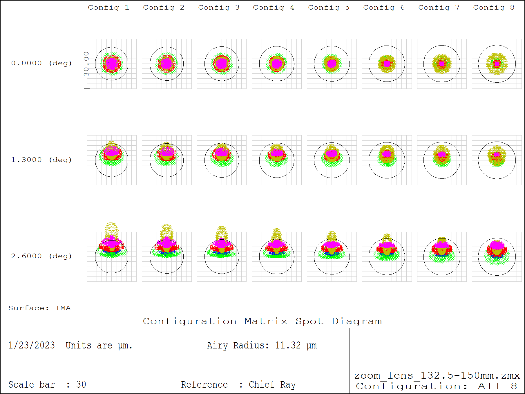
In Figure A1 we see the spot diagrams as a function of field (center to edge) and configuration (min to max focal length) across the visible spectrum (450-700nm). We can see that the system is mostly diffraction limited throughout the matrix, with some marginal degradation at the edge of the field for the shorter focal lengths (higher RR magnifications). In the interactive Figure A2 we show detailed views of the performance at the extremes of the range with configurations 1 and 8 (i.e. magnifications of 1.33 and 1.51). See zoom_lens.zip for more details (including Zemax files).
| Configuration: | Figure: |
Motion
Part of the design challenge in a zoom system is accommodating the motion of elements (or groups of elements). Here we adopt relatively large motions of all 3 lens groups from the PNP design. This has the drawback of being slower than small motions, but the benefit of loosening the opto-mechanical tolerances of the system, thereby allowing us to use stock optics and mechanics. In Figure A3 we see how we need to move the lens groups from the 'zero position' with a focal length of 132.5mm to the 'limit position' with a focal length of 150mm. The negative lens (center element in the design) moves the most by up to ~66mm, while the positive groups near the objective and the image move by up to ~18mm and ~42mm respectively.
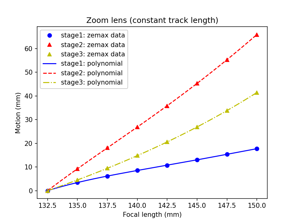
Below we provide the 'motion functions' that convert a requested focal length to a required movement of each lens or lens group (for driving linear stages or equivalent mechanics). Here's an example for a focal length of 140mm:
# Zoom_lens_132.5-150mm_motion.ods trendline polynomials
# Data from Zemax

def focal_length_to_lens_motion(f_mm, verbose=True):
    stage1_mm = (-     0.000103278288*f_mm**4
                 +     0.059929457484*f_mm**3
                 -    13.033982374525*f_mm**2
                 +  1260.150733009060*f_mm
                 - 45717.573446038600)
    stage2_mm = (-     0.000083979119*f_mm**4
                 +     0.049656589716*f_mm**3
                 -    10.961078884880*f_mm**2
                 +  1074.586675413890*f_mm
                 - 39574.398463973600)
    stage3_mm = (+    0.000018343468*f_mm**4
                 -    0.009692931167*f_mm**3
                 +    1.950506313956*f_mm**2
                 -  175.313955214666*f_mm
                 + 5879.390039196680)
    if verbose:
        print('\nf_mm = %0.2f'%f_mm)
        print('stage1_mm = %0.2f'%stage1_mm)
        print('stage2_mm = %0.2f'%stage2_mm)
        print('stage3_mm = %0.2f'%stage3_mm)
    return stage1_mm, stage2_mm, stage3_mm

# Input:
focal_length_to_lens_motion(140)

# Output:
## f_mm = 140.00
## stage1_mm = 8.52
## stage2_mm = 26.85
## stage3_mm = 14.78
Mechanics
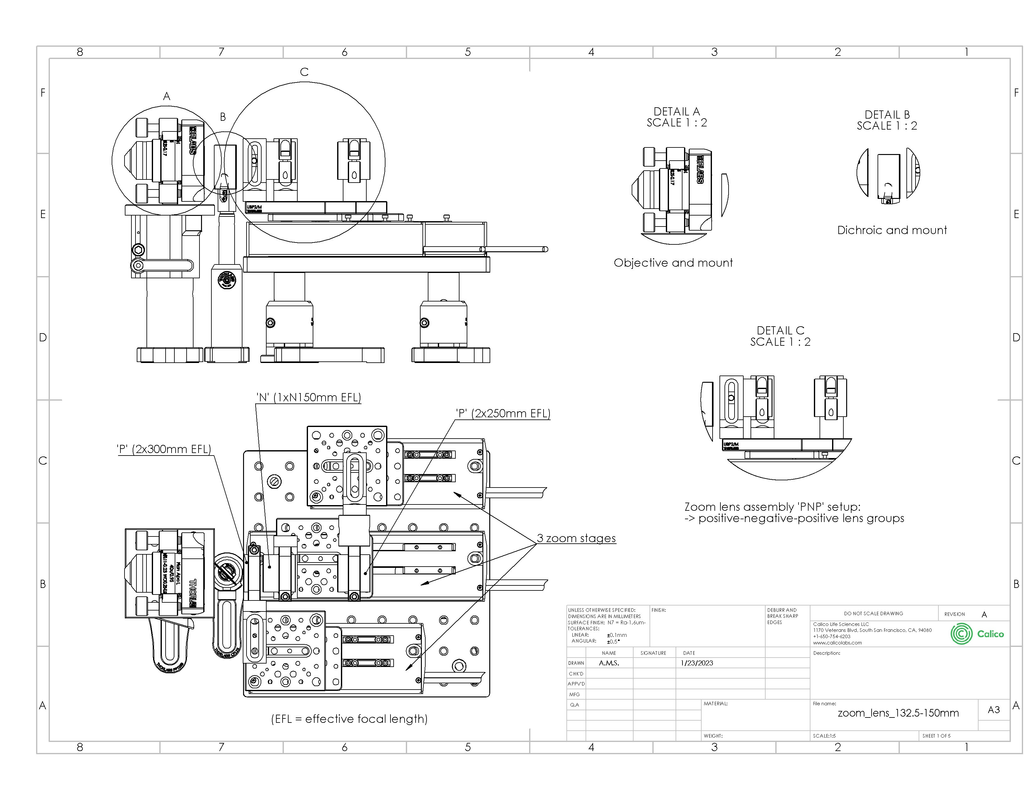
Here we offer a relatively simple mechanical design (Figure A4), that utilizes some fast 50-100mm linear stages from Thorlabs (parts DDS050 and DDS100). However, any mechanical solution that achieves the required alignment of the lenses and relative motions is acceptable. The solution we present combines the zoom optics into a single large mount that can be aligned to an axis that is parallel to the optical table, and includes provision for an objective and a dichroic. The DDS stages have a max speed of 500mm/s so we can expect a responsive zoom experience for tuning the magnification to different sample types. See the included zoom_lens_132.5-150mm.pdf for a high quality reproduction of the 2D drawings, or 3D CAD in eDrawings, Solidworks or .STEP format.
| Drawing: |
Alignment
The alignment of the zoom lens can be tricky, but with patience and good practice it can be done. For an experienced builder a morning or afternoon should be enough time. Here are some pointers:
- Setup a low power (~1mW) collimated laser beam with an adjustable diameter from ~1mm to ~10mm. A green laser beam like 532nm is preferred, since it has a central wavelength in the visible spectrum and appears bright to the human eye. Adjust the beam so it's horizontal to the optical table. Use the ~1mm beam for checking beam deviation and back reflections when aligning lenses to the laser beam. Use the ~10mm beam for checking the position of the focal planes.
- From the fully assembled 'PNP' zoom lens, remove the positive (P) lens groups, leaving only the negative (N) lens on the DDS100 motorized stage. Now iteratively adjust the 'XY' and 'tip/tilt' of the negative lens until the back reflections from the laser are centered on the ~1mm aperture. The back reflections should be symmetric over the full range of the zoom lens (~100mm here).
- Using a separate mount, align the positive lens groups to the ~1mm laser beam and check the back reflections. Because the positive groups consist of 2 separate achromats in a tube, it's possible for them to be poorly set and not share the same optical axis. This will show in the back reflections where no combination of 'XY' and 'tip/tilt' adjustment gives a clean and symmetric reflection. In this case the lenses need to be 're-seated' in the lens tubes. Loosening the lens retaining ring and giving a gentle shake of the lens tube in a vertical position seems to work. Some repetition may be needed.
- Now add the positive lens groups to the zoom lens assembly one at a time. For each lens group addition, repeat the iterative 'XY' and 'tip/tilt' alignment for that group (without changing the alignment of any other group), making sure the back reflection is clean over the full range of the zoom (~50mm here).
Control
Here's an example script for changing the focal length of the zoom lens across the full range (132.5-150mm). Before attempting to run this script, make sure the individual device adaptors for the DDS050 and DDS100 motorized stages are working, that the mechanical assembly is correct and the start positions of the stages are appropriate for the homing routine.
Testing
It's worth verifying the performance of the zoom lens before incorporating it into a system. According to the optical design, the 'Z' position of the front focal plane (FFP) and back focal plane (BFP) should be stable over the full range of the zoom. This can be tested in practice by observing a maximal 'speckle' pattern from some aluminum foil or a glass diffuser placed in the focus of the zoom lens (Figure A5). With this test we found the FFP and BFP tolerance to be better than +-100μm (see script and data here).
| Screen showing: |
Alternatively the focused laser spot from the ~10mm diameter beam can be imaged directly with a camera to confirm it's XY and Z location as the zoom lens is adjusted over the full range (Figure A6). Here we performed this test by sweeping a small camera through the focus for each of the 8 Zemax configurations (see acquisition script). With this setup we also found the maximum FFP and BFP deviations to be less than +-100μm, and XY deviations in spot position to be less than ~40μm. Better results may be possible with more thorough alignment. Download FFP_data.zip and BFP_data.zip to see the data and run the scripts that estimate the focus position.
If we assume a 40x magnification for the base microscope then a 40μm XY deviation in the image plane corresponds to a ~1μm XY shift in the sample (40μm/40), and a 100μm Z deviation in the focal plane to a ~60nm Z shift in the sample (100μm/40^2). Note that the maximum numerical aperture for the zoom lens is ~0.38 (5/132.5), and so the +-100μm result is within the traditional depth of field of ~370μm (0.532/0.38^2).
Large FOV SOLS
Current prototype
On the road to building an 'any immersion' large FOV SOLS microscope we opted to build a 'static' configuration (i.e. no zoom lens) to show the potential of the new approach. The system was built to accommodate primary objectives with a 5mm effective focal length (i.e. the Nikon 40x family) with a remote refocus tuned for watery samples (i.e. a sample RI of 1.33). The transition from air to water immersion is one of the most extreme examples of an RI mismatch and so the Nikon 40x0.95 air and 40x1.15 water objectives were chosen as options for the primary objective. The last microscope (often referred to as microscope 3 in a SOLS design) was tilted to 50deg to accommodate the NA of both the air and water objectives. A simple cylindrical lens light-sheet excitation path was assembled, and combined with the following emission path optics:
| Item | Supplier | Part | Description |
|---|---|---|---|
| S | Biologist | Sample | preferred refractive index: 1.33 |
| O1 | Nikon | MRD77410 or MRD00405 | CFI Apo LWD Lambda S 40XC WI (NA=1.15) or CFI Plan Apo Lambda 40XC (NA=0.95) |
| TL1 | Nikon | MXA22018 | Tube lens, EFL=200 mm |
| SL1 | Thorlabs | TTL100-A | Scan lens, EFL=100 mm |
| G1 | Thorlabs | GVS211/M | 1D Galvo system, ∅10 mm, E02 coated |
| SL2 | Thorlabs | TTL100-A | Scan lens, EFL=100 mm |
| TL2 | Thorlabs | AMS custom | Tube lens, EFL=300 mm |
| D | Chroma | ZT405/488/561/640rpcv2 | Quad band dichroic |
| O2 | Nikon | MRD00205 | CFI Plan Apo Lambda 20XC (NA 0.75) |
| O2* | Carolina | 633037 | Cover Glasses, Circles, 25 mm, Thickness 0.13-0.17 mm |
| O3 | ASI | AMS-AGY v2.0 | Special glass tipped objective (a.k.a. KingSnout) |
| E | Chroma | ZET405/488/561/640m | Quad emission filter, ∅25 mm mounted |
| TL3 | Thorlabs | TTL200MP | Tube lens, EFL=200 mm |
| C | PCO | edge 4.2 cl | sCMOS camera, 2048x2048 px, 6.5μm pitch |
Data
The Python scripts that were used to run the microscope and process the data are included in the 'data' folder (download full repository). The microscope was aligned on a best effort basis, with an overexpanded Gaussian beam for the light-sheet input (wasteful but gave uniform illumination). The light-sheet was generated with a 1mm slit aperture just before the cylindrical lens which was mapped onto the O2 back focal plane with a 1:1 relay (so about 0.66mm at the O1 BFP in this configuration). The PSF data was processed with the same method as here (which includes sample data). To avoid bloat the raw data (~500GB) is not included here so the publication can be readily stored and circulated offline.
Improved configuration
Some attractive upgrades to the current prototype include:
- Adding the zoom lens to allow continuous tuning of the remote refocus volume to the sample RI (which we expect to keep the light-sheet in better alignment).
- Swapping O2 from the Nikon 20x0.75 air objective to the 40x0.95 air objective. This gives improved collection from higher NA primary objectives, and the 40x has the correct effective focal length (5mm) to pair with the zoom assembly.
- Using a high quality coverslip at O2. ASI currently offers the Nikon 40x0.95 air objective with a high quality (AR coated) coverslip glued to the front.
- Adjusting the focal length of tube lens 3 for a good compromise on the Nyquist pixel size (something like a 250mm EFL).