Microscope objectives
An introduction to 'infinity' corrected microscope objectives.
ContentsPoint spread function
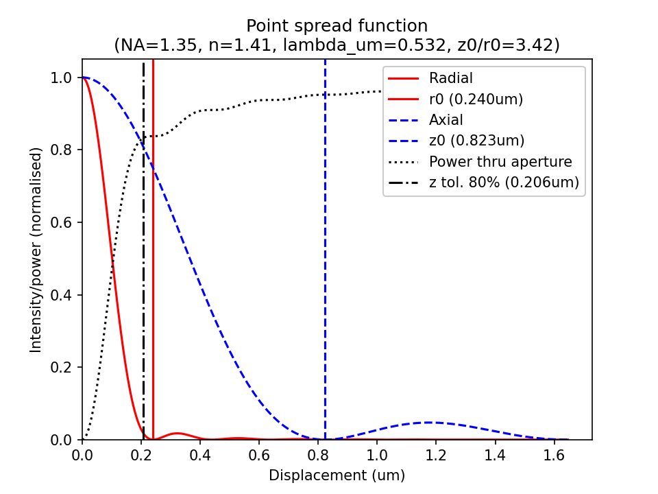
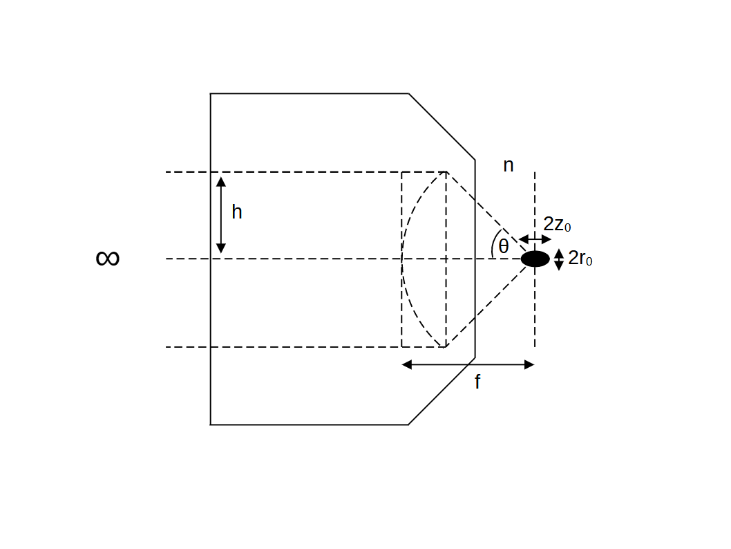
From Born 2019, the diffraction limited intensity distribution near focus is given radially (i.e. in the image plane) by: \[ I(v,0) = I_0 \left( \frac{2J_1(v)}{v} \right)^2 \tag{1}\] and along the optic axis by: \[ I(0,u) = I_0 \left( \frac{\sin(u/4)}{u/4} \right)^2 \tag{2}\] where, \[ v = \frac{2 \pi h}{\lambda f}r \tag{3}\] and, \[ u = \frac{2 \pi h^2}{\lambda f^2}z \tag{4}\] where \(J_1\) is the Bessel function (for n=1) and it has been assumed that \(f \ll h \ll \lambda\) and \(\lambda f \ll h^2 \) (which may not be strictly true for many objectives). In the case of infinity correction we can make the substitution \( \frac{h}{f} = \frac{NA}{n}\) into (3) and (4) (where we have implicitly used \( \frac{n_i}{f_i} = - \frac{n_o}{f_o}\)) , and convert to the vacuum wavelength \( \lambda_0 = n \lambda \) to give: \[ v = \frac{2 \pi NA}{\lambda_0}r \tag{5}\] and, \[ u = \frac{2 \pi NA^2}{n\lambda_0}z \tag{6}\] For the radial intensity (1) the first zero \(r_0\) occurs at \(v = \pm 1.22 \pi \) and for the axial intensity (2) the first zero \(z_0\) occurs at \(u/4 = \pm \pi \). So substituting into (5) and (6) we see that: \[ \pm 1.22 = \frac{2 NA}{\lambda_0}r_0 \tag{7}\] and, \[ \pm 1 = \frac{1}{4} \frac{2 NA^2}{n\lambda_0}z_0 \tag{8}\] which we can rearrange to the familiar forms: \[ r_0 = \pm 0.61 \frac{\lambda_0}{NA} \tag{9}\] and, \[ z_0 = \pm 2 \frac{n \lambda_0}{NA^2} \tag{10}\]
The first radial minimum \(r_0\) is often referred to as the Airy radius, and is also the Rayleigh limit of resolution (\(r_{min}\)) in a diffraction limited image: \[ r_{min} = r_0 \tag{11}\] For the axial intensity, it is traditional to take the focal tolerance \(\Delta z\) to be the point at which the intensity has decreased by 20% (like the diffraction limit for the Strehl ratio), which occurs at \(u \approx 3.2 \): \[ \pm 3.2 \approx \frac{2 \pi NA^2}{n\lambda_0} \Delta z \tag{12}\] If we allow \( 3.2 / \pi \sim 1\) then: \[ \Delta z \approx \pm \frac{1}{2} \frac{n \lambda_0}{NA^2} \tag{13}\] So finally we see the definition for the traditional depth of field (\(DOF\)), the range over which the image appears 'in focus': \[ DOF = \frac{n \lambda_0}{NA^2} \tag{14}\] If we apply the Rayleigh limit of resolution in the axial direction, then \(z_{min} = z_0\), and we see that the smallest axial feature size we can resolve is twice the depth of field: \[ z_{min} = 2 DOF \tag{15}\] Note: Equations (11) and (15) are the generally accepted as the limits on resolution for an objective lens (Pawley 2006).
In addition to radial intensity (1), it can also be useful to know the integrated power through a circular aperture (Born 2019): \[ P(v,0) = P_0 (1- J_0(v)^2 - J_1(v)^2) \tag{16}\] (which is about 84% for an aperture of radius \(r_0\))