Microscope objectives
An introduction to 'infinity' corrected microscope objectives.
ContentsCollection
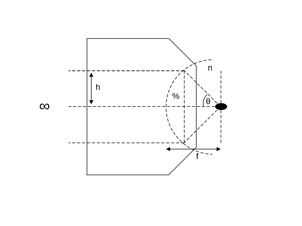
An ideal point emitter generates a spherical wave of uniform amplitude, with total surface area (Larson 2014): \[ A_{sphere} = 4 \pi r^2 \tag{1}\] For an objective that respects a planar boundary (image plane) then the maximum possible collection area \(A_{max}\) is the area of a hemisphere: \[ A_{max} = 2 \pi r^2 \tag{2}\] The actual area collected is of course limited by the collection half angle (\(\theta\)) to the area of a spherical cap (Polyanin 2006): \[ A_{collection} = 2 \pi r^2(1 - \cos\theta) \tag{3}\] So the collection of an objective normalised to the hemispheric maximum is simply: \[ \frac{A_{collection}}{A_{max}} = 1 - \cos\theta \tag{4}\] If we rewrite (4) in terms of \(\sin\theta\): \[ \frac{A_{collection}}{A_{max}} = 1 - (1 - \sin^2\theta)^\frac{1}{2} \tag{5}\] and now use the Taylor expansion of the form: \[ (1 - \sin^2\theta)^\frac{1}{2} = 1 - \frac{1}{2} \sin^2\theta \; - \; ... \tag{6}\] then we can rewrite (5) as: \[ \frac{A_{collection}}{A_{max}} \approx \frac{1}{2} \sin^2\theta \tag{7}\] Or in terms of numerical aperture as: \[ \frac{A_{collection}}{A_{max}} \approx \frac{ NA^2}{2n^2} \tag{8}\] So all things being equal, the brightness of an image is approximately proportional to the numerical aperture squared (Pawley 2006): \[ brightness \propto NA^2 \tag{9}\] Note: the approximation by Taylor series to express the brightness in terms of \(NA\) seems unnecessary given the elegance of the \(1 - \cos\theta\) expression, and the approximation gets worse for higher half angles (\(\theta\)). However, this simple treatment gives no consideration to reflection losses throughout the many elements that make a high \(NA\) objective, and the higher angle rays are the most affected, which somewhat justifies the regular use and convenience of (9).