amsikking: Microscope objectives

Band limit

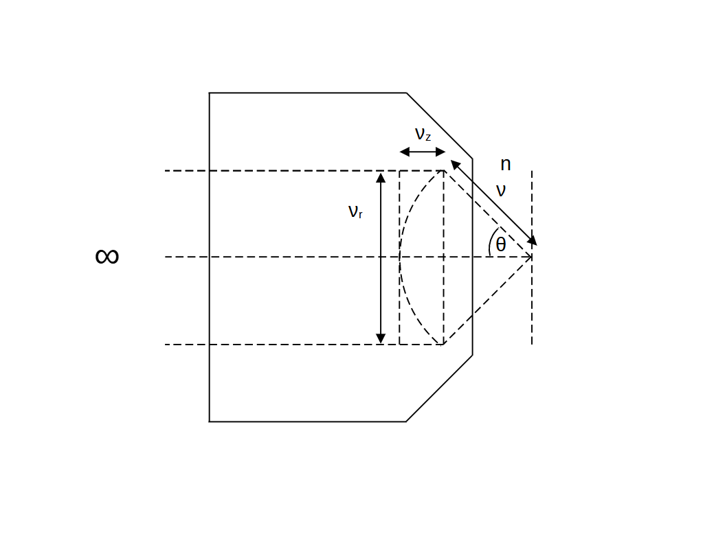
Inspired by McCutchen 1964, if we assume the highest spatial frequency \(\nu\) of an object that we can measure is the inverse of its emission wavelength \(\lambda\), then we can write: \[ \nu = \frac{1}{\lambda} \tag{1}\] or, \[ \nu = \frac{n}{\lambda_0} \tag{2}\] where \(\lambda_0\) is the vacuum wavelength and \(n\) is the refractive index of the medium.

If we now accept that the back focal plane of an objective resides in reciprocal space (i.e. the fourier transform of the object) and that (due to the infinity correction) the back focal plane of the objective has the shape of a spherical cap, we can see from the diagram below that: \[ \nu_r = 2 \nu\sin\theta \tag{3}\] and, \[ \nu_z = \nu (1 - \cos\theta) \tag{4}\] where \(\nu_r\) and \(\nu_z\) are the highest spatial frequencies we can measure in the radial and axial directions respectively, i.e. they are the band limit.

We can now return to real space by rewriting (3) and (4) in terms of the minimum feature size \(r_{min} = \frac{1}{\nu_r} \) and \(z_{min} = \frac{1}{\nu_z} \): \[ r_{min} = \frac{\lambda_0}{2 n \sin\theta} \tag{5}\] and, \[ z_{min} = \frac{\lambda_0}{n(1 - \cos\theta)} \tag{6}\] Equation (5) is immediately recognizable as the Abbe diffraction limit for a microscope, which we can rewrite in terms of the numerical aperture as: \[ r_{min} = \frac{\lambda_0}{2 NA} \tag{7}\] We can also convert equation (6) to a more familiar form by first rewriting in terms of \(\sin\theta\): \[ z_{min} = \frac{\lambda_0}{n(1 - (1 - \sin^2\theta)^\frac{1}{2})} \tag{8}\] and then using the Taylor expansion of the form: \[ (1 - \sin^2\theta)^\frac{1}{2} = 1 - \frac{1}{2} \sin^2\theta \; - \; ... \tag{9}\] So to 2nd order: \[ z_{min} \approx \frac{\lambda_0}{n (\frac{1}{2} \sin^2\theta)} \tag{10}\] Or in terms of numerical aperture: \[ z_{min} \approx \frac{2n\lambda_0}{NA^2} \tag{11}\] which is twice the traditional depth of field: \[ z_{min} \approx 2 DOF \tag{12}\]